HTML Character Entities.     If "α" does not display as a single character then please read this note:
This document makes use of the HTML character entities in its text, so if your browser does not support them you will see the raw HTML tags which call them up. I believe that the text should display properly for browser versions starting from v4.5 for Internet Explorer, v6 for Netscape and v6 for Opera.

**    Summary

This paper studies sensitivity and noise in the detection of small movements of an electronic image when the detection algorithm uses inner products of image vectors. This is related to the so called "Doppler" methods of surface image velocity measurement. It deals essentially with the case of a one dimensional image, offering comments regarding the generalisation of the results to two dimensions. The mathematics used is couched as far as possible in terms of the properties of smooth functions over finite domains (i.e. with no significant structure in either infinite or infinitesimal regions of their domains). This leads to a characteristically engineering style in which the concerns over approach to mathematical limits are deferred until after manipulation of the structure of the model.

The "Document ident" shown just below the header of the paper and showing date of last update should be used to check for the specific form of the paper, in cases where that might matter. Please communicate comments to Tony Booth - for email see foot of AGB home page.

Contents

**     Motivation
**     Establishing a Model
**     Dynamic and Quantisation Errors
**     Process Sensitivity and Intrinsic Noise
**     Filter Optimisation
**     Uniform Sensitivity
**     Generalisation to Two Dimensions
**     Some Typical Results
**     Discussion
**     References and Background Reading
 

**    Motivation

The recent development of economical electronic camera chips has made it attractive to infer various sorts of measurements by processing video image signals. One form of such processing is that which produces a signal to represent the magnitude of small movements of an image between successive video scans. The motivation for this is to transduce movements using only the given texture such as may be found in the microscopic image of a surface or the speckle image produced by coherent illumination. The advantage of measurements performed in this way is that no specially precise preparation of the observed object is necessary as would be the case if using say graticule markings or interference fringes.

Techniques for the tracking of patterns became important in the development of radar and non-contact speed measurement, where the delay between two observed stochastic signals would vary (refs Spilker & Magill [SM61], H.Meyr [HM76]). More recently similar concerns have arisen in the fields of general image processing (refs Webber & Delashmit [WD75], Horn & Schunk [HS81], Bresler & Merhav [BM87]) handling parallel arrays of signals which are discrete in space, and when processing is digital, also discrete in time. It is this discrete array form of the problem which is addressed here, and in particular the detection of incremental movements up to about the spatial sample size (pixel spacing).

The earlier related work deals with the calculation of sensitivity, but does not arrive at an analytical model for the noise in the measurement. This latter is particularly interesting because these algorithms produce an inherent noise due to self interaction of the image being observed which is additional to any noise caused by original errors of image observation. The work of H.Meyr [HM76] points out the essential nature of the intrinsic process noise, but his analysis is applied to a more limited model than the bilinear process discussed here, and also his treatment of the nature of the process noise spectrum gives only an initial outline, and does not use the technique of convolution in the frequency domain as applied here.

**    Establishing a Model

The detection of pattern movement is a second order process of recognition in the sense that the pattern being handled is not given a priori, but rather it is to be established as part of the observation process using different points in time. We must seek a class of processes in which the interaction of at least two bodies of data occurs. The lowest order of nonlinear operation capable of contributing such a result is the product of two original observations, and thus the field of quadratic functions of observed vectors suggests itself.

Exclusion of terms of order higher than quadratic in the data is by no means fundamental in estimating motion. A simple counter example is the use of search strategies seeking high levels of correlation under spatial shifts of earlier observations (ref I.Yamaguchi,T.Fujita [YF91]). However, for the detection of small movements the use of a constant structure algorithm (i.e. avoiding logical branching such as in searching) is often possible and desirable. Amongst these constant structure algorithms the class of functions built from weighted sums of products of pairs of measured scalar data values is attractive both from the point of view of regularity of implementation and also in being reasonably amenable to analysis of its performance.

	General Bilinear Operation upon Two Data Vectors.

Product terms in which both factors are data obtained at the same instant cannot contribute to an estimate of movement and we would like to obtain an estimate from observations at just two points in time. Because of this the algorithm should best be homogeneously bilinear, that is having every additive term linear in each of two sets of data. It leaves the rôle of temporal self products to be found only in the computation of sensitivity and the optimisation of algorithm weights.

The complete form of an estimator algorithm must in general consist of more than just a constant structure constantly weighted sum of products of pairs of scalar data values because some allowance has to be made for differing amplitudes and statistical forms of the observed pattern. However, the considerations affecting the sensitivity can be separated from those concerned with the evaluation of individual estimates of movement. For example, it is possible at least to calculate a sensitivity factor for the overall algorithm independently and rather more slowly (less frequently) than the individual estimates of movement. In a more advanced form of the algorithm it might also be desirable to tune the weights for the bilinear products to optimise the quality of the estimation (e.g. to minimise errors versus motion sensitivity), but again this can usually be performed independently and more slowly (less frequently) than the estimations of the movement itself.

We may need to take care to distinguish the more basic concept of an underlying physical function f(x), which cannot be directly observed, from g(x) which is observed by sampling through a window weighting function. They are both continuous functions of the pattern spatial domain, but the physical function is usually to be expected to contain greater power in the higher frequencies of its spatial power density spectrum than would any observed function seen through a spatial averaging sampling window. For the purpose of calculating sensitivity it is not necessary to handle the lower level process of sample taking, but only its results in the form of sample values, and hence the function symbol g(x) as distinct from f(x). On this basis the samples u(n, x) each correspond to a value of the function g(x) at a particular value of x but offset to the nth sample window pitch position.

A matrix expression of the general bilinear form is as follows:

v   =   u₀^TAu₁(ξ)

where
u₀ is a reference measurement vector of order N,
u₁ is a similar measurement vector of order N, but physically displaced by ξ,
v is a scalar estimate result,
and
matrix A of order N × N contains all of the coefficients controlling dependence of v upon observations.

From the required properties of the motion detection process it is possible to restrict this expression further. Firstly we can nearly always simplify things in practice by allowing the correlative statistical definition of the vectors u₀ and u₁ only to be symmetrical about the origin (i.e. even functions) of spatial offsets. Further, results obtained for positive displacements must be of equal magnitude and opposite sign to those obtained for the corresponding negative displacements (i.e. v must be an odd function of displacement). From these restrictions it follows that the matrix A must be anti-symmetric, so for its individual elements:

a_i,j   =   −a_j,i,     a_i,i   =   0     for all   0 < i, j ≤ N

By splitting this anti-symmetric matrix A into upper and lower triangles U and −U^T respectively, so that A = U − U^T, we can write:

v   =   u₀^TUu₁(ξ) − (u₁(ξ))^TUu₀

Where the vectors are of high enough order N so that the spatial limit of autocorrelation L is less than N the matrix U is a diagonal band with width L−1 of non-zero values above its zero major diagonal. This is still a rather high order model of the algorithm for practical purposes. It can for instance accommodate variation of the relative importance of the contributions along the length of the vectors u₀ and u₁. As a special case which is commonly valuable, the relative importance can be taken to be weighted according to a simple function or even to be uniform along the lengths of these vectors. In the latter case the matrix U contains constant values along the various diagonal stripes (i.e. it is a Töplitz matrix), so that:

a_{i, j}   =   a_{(i+k), (j+k)}     for all 0 < i, j, (i+k), (j+k) ≤ N

Under this latter restriction the bilinear form can be approximated by a discrete convolutional filter form of expression which is economical to evaluate. In this form it is then necessary to decide what is to be done with the overlapping terms at the ends of the otherwise repetitive local calculation, but as N increases for a given L this aspect of approximation improves. Using h(ν) as the discrete filter weighting function defined over the range −L ≤ N ≤ L then because of the simplicity of the Töplitz anti-symmetric form of the matrix, h(0) = 0, h(ν) = −h(−ν) and this function is related to the matrix elements by:

h(ν)   =   a_{i, (i+ν)}     for any 0 < i, i + ν ≤ N which exists.

A convolutional approximation of the algorithm may then be written as:

This expression is compact and also suggests how to mechanise the algorithm. Alternatively if either symmetry with respect to the treatment of u₀ and u₁ is required or one-sided spatial filtering is preferred then a similar but not quite identical approximation is available as:

These expressions differ in the way that they truncate some overlapping convolution terms at the ends of the vectors. There are other possible choices of which terms to drop, possible apodising functions (graded weighting of the end terms) and there is a need to assess the error characteristics of any such chosen approach.

For the cases where the spatial autocorrelation function of the data vectors may be neglected beyond the region of one pixel it is possible to achieve useful performance with the function h(n) simplified to the single term h(1) only. This simplifies the above expression to:

In this case there is also another useful form of the convolutional expression which at the cost of losing one more term in the length of the vector reduces the need for storage of prior results from u₀ from two vectors to only one of which the elements are local spatial differences. By this means the sometimes large unwanted terms in low spatial frequency are not then stored:

This is equivalent to the order of model considered by H.Meyr [HM76], though he also proposes prefiltering the factor signals to give some degree of optimisation.

**    Dynamic and Quantisation Errors

A further question regarding choice of structure of mechanisation of the algorithm arises in connection with the effects of dynamic noise in the data and quantised coding of either the original data or the bilinear products prior to their weighted summation. Although the algorithm may be viewed overall according to its basic bilinear nature, still it may be necessary to carry out algebraic operations (in particular, the forming of differences) either prior to first quantisation of the data or at least very early in the flow of the process if we are to avoid having to encode, store, transmit and process relatively large terms which will eventually be removed by subtractive cancellation. This is a difficult area to resolve in a general way because the importance of avoiding such differences of large quantities depends upon the statistical nature of the pattern being observed and the form of the result desired. Unless estimated values of measurement and coding quantisation noise are introduced to the model, then any noise minimising type of optimum filter design will not be sensitive to its presence at all, and in that case it will indicate that all structures of the solution are of equal performance, equivalent to the case with pure additions and multiplications of real numbers in the bilinear algorithm.

**    Process Sensitivity and Intrinsic Noise

In the usual situation where the underlying physical function has a detailed random nature the estimates obtained around any particular reference point are subject to an error which is a static random function of space (as well as any dynamic errors of observation which are ever present). This source of static error may be regarded as caused partly by the sampling distribution of the spatial variance which contributes to the result, and partly by the aliasing of high frequencies in the underlying physical form of the surface (a continuous function of spatial co-ordinates) into the data by the spatial weighting function form of the sensor pixel sample windows.

The situation with optically produced speckle.

In the case of optical array sensors detecting speckle patterns the form of these windows can often be regarded as approximately rectangular due to the simple structure of the boundaries between adjacent pixel sensing regions, and therefore this function cannot be readily controlled. However it is often possible to arrange the optical system so that the combination of wavelength and aperture limits the range of spatial frequency in the speckle pattern. If the illumination spot diameter is the effective aperture limiting factor then it can be set to create this limit, and by arranging for the edges of the spot profile to taper smoothly (say roughly in a Gaussian form) the higher frequencies can be made to taper away smoothly as well. If the size of the illumination spot cannot be reduced sufficiently to impose the required spatial cut-off frequency then the only remaining resort to achieve this type of spatial filtering is to bring the spot into focus somewhere in the transmission path and at a plane near to that focus apply an additional aperture restriction limiting the diameter of the spot utilised. However, this technique wastes luminous power.

If the structure of the scattering surface is confined to spatial frequencies below that of the illumination wave and/or it has too low an index of depth modulation then the scattered light will be delivered closer to the path of specular reflection than would correspond to the cosine form of Lambert's law for an idealised scattering surface. If this effect is sufficiently strong then it will become an aperture limiting effect, with the consequence that the speckle produced will suffer a loss of high frequencies according to the usual Fourier transform relationships. Surface structure with periodic regularity will cause concentration of scattered radiation at angles offset from the specular reflection path, and if these fall within the observation aperture they will produce narrow aperture effects at angles offset from the specular reflection path centre.

We need an analysis of the bilinear movement transduction process which can yield both an estimate of the sensitivity, and also of the dispersion of the results about the expected value. It might be conceived as a spatial variance density spectrum Ψ(ω, h) which is a function of spatial frequency ω of the output of the estimation process and of the displacement h being observed, and averaged over the spatial locations x of the observation.

A sample window summation weighting function w(ξ) operates on a physical function f(x) to produce a sample value g(x). A vector of these samples u(n, x) is formed as a regular array over the physical domain with pitch P and located at position x. One such sample vector u(n, x) is to be multiplied element by element by another u(n, x+h) obtained similarly but shifted by a continuous interval h, and spatially prefiltered by a linear convolutional filter h(ν). The product vector is then to be summed element-wise under a determinate weighting function a(ν) of the discrete sample position variable ν (thus a(ν) is an apodising function). The function g(x) is characterised only to the extent of information regarding its autocorrelation function γ(ξ), or equivalently of its power density spectrum Γ(ω). The filter function is determined in terms of its discrete impulse response h(ν), or equivalently of its periodic continuous frequency response H(ω). The function a(ν) is of significant magnitude over only a finite contiguous region of its argument −N/2 < n ≤ N/2 and its Fourier transform is therefore periodic with period NΩ = 2π/P and can be expressed as a finite series of N terms. Thus the index variables for both the physical and frequency domains of these discrete functions may operate to modulus N so long as no significant product terms are derived across the boundary corresponding to the physical limits of the observed array. For most cases of interest a similar structure applies to the function h(ν), but the case considered here treats the Fourier transform H(ω) as having a continuous domain because it is used in conjunction with the physical domain variable under continuous shifts.

In the following:

ξ(f(ξ), ω)	denotes the Fourier transform with argument ω over domain ξ
x(f(x), ξ)	denotes the autocorrelation function with shift argument ξ averaged over domain x and
x(f1(x), f2(x), ξ)	denotes the cross correlation function from f1(x) to f2(x) with shift argument ξ averaged over domain x.

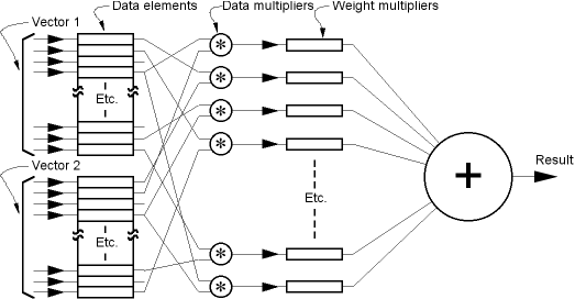
The computational structure of the estimation mechanism is:

E1

where ν, μ operate to modulus N, and x is the unbounded continuous physical position variable.

Using Av_x as the operation of forming an average over the domain x, the required calibration estimator is then:

E2


.... and the spectral distribution of variance (total of signal and error) over the x domain is:

E3




.... where determinate relationships are:
	A(νf) and a(νa) both real, even, over finite discrete domains.
H(ω)   =   ν(h(ν), ω, P, N)	h(ν) real, odd, finite significant extent over infinite discrete domain. H(ω) imaginary, odd, periodic at interval NΩ = 2π/P over continuous domain.
.... and stochastic relationships are:
Γ(ω)   =   ξ(xg(x), ξ), ω)	Γ(ω) real, even, finite significant extent over infinite continuous domain. g(x) band limited, random, infinite extent.
u(n, h)   =   g(n.P + h)	Sampled signal shifted by continuous h.


In this case random means that there is no model available by means of which to predict any part of the said function better than is possible using the spectral (or equivalent autocorrelative) relationships given.

From equations E1 and E2 an expected (mean) value of the estimate may be written as:

	E4
ω continuous modulo NΩ

From equations E1 and E3 a spatial spectral analysis of the variance may be obtained as:

E5

We now construct an expression Ψ(ω, h) leading to the above spectrum by integrating products of all pairs of narrow band terms with a given difference of frequencies because they will contribute coherently to a single narrow band of the spectrum. This integration operation is a convolution in the frequency domain. Because the terms add coherently the resulting expression is in the nature of a wave function and will need to be squared to produce the spatial power density spectrum of the product signal:

Ψ(ω, h)   =   (ψ(ω, h))²

A feature of the wave function Ψ(ω, h) is that it represents in its lower frequencies the signal terms required for measurement since these are the coherently added products of like frequency components from the two factor signals. Thus the sensitivity of the system can be obtained as:

The frequency domain convolution may be constructed by using an abstract narrow band filter operator (φ(x), ω, ζ) with centre frequency ω and bandwidth ζ and with convolutional capability (i.e. a requisite normalised orthogonality and zero phase). We estimate the spectral amplitude wave function as an integral of coherent products of different frequency components of the data following the form of the expression in E5:

ω continuous, μ, ν, α discrete modulo N, β continuous modulo NΩ

.... where frequency index α and frequency β are convolution parameters. Note that the integration over β is "coherent" in that the integrand is the product variable, not its square. This integrand is not necessarily always positive. The 1/(ω − αΩ) factor effects a summation in the physical domain which is subject to the weighting function a(ν).

Removing the filter and delay effects from the operation of infinite averaging:

The average over x is a real even function of β. Therefore so long as H(β) is an imaginary odd (or as a matter of fact, any Hermitian) function the integration over β will yield a real result.

So long as sufficient reduction to a narrow bandwidth ζ is valid under the assumption of stationary statistics then this approaches:

E6

ω continuous, β continuous modulo NΩ

 
... or alternatively, using symmetry of even functions to allow integration over a half period:

ω continuous, β continuous in 0 < β ≤ NΩ/2

The spatial spectral power density is then obtained as Ψ(ω, h) = (ψ(ω, h))², and an estimator for the mean output of the process as a function of h which also agrees with E4 is:

E7

ω continuous, β continuous modulo NΩ

 

**    Filter Optimisation

In order to estimate small movements the process can be viewed in a differential form. Obtaining the best estimate of movement is then determined by obtaining the best estimate of the spatial gradient in the vicinity of each point observation (as the first term in a Taylor series). Assume we are given only some information about the autocorrelation function _x(g(x), ξ) of point samples of the pattern g(x), these correlations being taken over a continuously variable shift interval ξ.

There follows an analysis of the bilinear convolutional class of algorithms in relation to their specific ability to interpolate very small pattern movements, less than the sample pitch, around some reference pattern sample which is undefined, but for which we are given some information of spatial correlations. This form of the problem has maximum sensitivity to the influence of quantisation and other errors caused by handling large redundant terms in the original data, but at the same time reduces the complexity to the equivalent of the design of the statistically optimum linear filter weighting function h(ν). It would, of course, not necessarily be a good basis of design for a system which is not concerned with such small movements.

Using P as the pitch of the sample array, u(n, x) can be defined in value by:

u(n, x)   =   g(x + n.P)

An estimate of expected gradients (n, x) of the observed pattern at the sample points for the one dimensional case may be obtained from the samples u(n, x) by a linear estimator of the form:

where h(q) is designed to suit _x(g(x), ξ), and by symmetry of the autocorrelation function h(q) is an odd function.

The cross correlation function between the original function g(x) and its first derivative g'(x) can be derived from the autocorrelation as:

To work with a mixture of discrete and continuous domain variables we use symbols:

n(a(n), q)	Discrete autocorrelation function of a(n) over discrete shift q.
n(a(n), b(n), q)	Discrete cross correlation function from a(n) to b(n) over discrete shift q.
n(a(n), ω)	Fourier transform of a discrete operand a(n) over the continuous frequency domain ω, sample pitch P determining −π/P < ω ≤ π/P.

In seeking to design the slope estimator filter coefficients h(q) the Wiener-Hopf equation (ref H.V.Poor [HP94]) in terms of discrete domains offers the following formulation for the optimum (i.e. least mean square error) discrete linear filter weighting function (q) based upon discrete auto and cross correlations, and this can be used for estimation of the local derivative with respect to movements about a given pattern reference:

These functions defined only at discrete points which are necessary as the result of a sampling process contain less information than can be expressed in the continuous domain, and in particular can only represent part of the information which may be expressed in the presumed given autocorrelation function of g(x) and the derived cross correlation between it and its slope g'(x). Adhering to the reduced information contained in the discrete form of the Wiener-Hopf equation above we can find expressions for the discrete cross and autocorrelations required in this expression from the presumed given autocorrelation of the continuous function as follows:

Substituting in the Wiener-Hopf formula for the best filter estimator of the derivative:

Expressing this by summing the aliased frequency terms:

In this simple case with no quantisation or dynamic noise added, it is possible to simplify this further if the surface spatial bandwidth determined by g(x) is sufficiently small to make the alias terms negligible under the multiplier ω + k/P. The filter then reduces to a simple differentiator. Otherwise it requires detailed evaluation.

For the case where dynamic noise is added to the observed signals it may be considered as having correlations in either or both of space and time. These can be built into the Wiener-Hopf equation accordingly. However an important simple form of noise is that which has no correlations in either space or time, i.e. which is white in both of these domains. This has the effect of adding a constant term of power at every frequency in the denominator of the Wiener-Hopf equation for the optimum spatial filter, but has no effect upon the numerator. If this constant term is large enough to dominate the autocorrelation then the denominator becomes approximately constant. For this case of low signal to noise ratio the optimum filter becomes directly dependent upon the spatial autocorrelation:

Again this case will simplify so long as the aliased frequency terms can be neglected, giving then the optimum filter directly except for a gain constant as:

**    Uniform Sensitivity

Rather than seek to optimise the signal to noise ratio of the process there might be advantage in setting up the filter to give the calibration a degree of independence of the statistics of the observed spatial function. If the variance is taken to be the easiest parameter against which to compensate for changes then it would be desirable to make the filter produce a sensitivity which is independent of spatial spectral colouration of the physical data at any given variance. By reference to equation E7 above it may be seen that to achieve this requires that the sensitivity of the filter shall remain constant at all frequencies except for a step of sign reversal at the origin of frequency. Because we are dealing with a sampled system there must be another step reversal of sensitivity at the finite Nyquist frequency (half the spatial sampling frequency). A filter impulse response with this frequency characteristic has all even terms zero, and the coefficients for the odd terms are proportional to the reciprocals of their respective orders: h(ν) = k/ν for odd ν, and h(ν) = 0 for even ν.

Practical adjustments close to this form of filter therefore offer valuable characteristics. Furthermore, if any correlations can be found within the spatial spectral structure of the underlying physical function then some other compensating shaping of the filter in the spatial frequency domain can possibly offer a further reduction in changes of sensitivity in the face of varying statistics.

**    Generalisation to Two Dimensions

Schemes for the detection of image motion can be implemented in higher dimensional spaces than the one dimension as analysed above. The burden of calculation in implementing or numerically analysing such a measurement increases exponentially with the number of dimensions, but the analysis can be kept to a similar form to that used for one dimension, but using higher orders of integration and summation.

In order to invoke the Fourier analysis at all we must use a basis for our analysis of functions which is composed of orthogonal simple harmonic functions. The foregoing analysis does this in the conventional way in one dimension. To correspond to a rectangular array of sampling points we may use a Cartesian scheme with each analysis co-ordinate axis being one of the two natural grid axes, and seek a resolution of the result velocity into these two orthogonal directions in the image plane. We may use the parameters of x-frequency ω and y-frequency υ in:

Equations E6 and E7 can both be generalised to vector form. To do this both the integral and the summation operations must be raised to the order of the vector space. The h·β product in the argument of the exponential function and correspondingly the h·ω argument of the sine function must be treated as the inner products of their vector factors. Γ(ω) is a real scalar function of its vector argument. The filter weighting function h(ω) must take a vector value and each element of its vector Fourier transform H(ω) must then be imaginary and must be odd in the corresponding vector element of ω but even in all other elements.

Recalling equations E6 and E7 and adding dots where inner products are required for vector multiplications:

E8




E9

The designer has here a greater range of choice of the form of h(ν) and hence of H(ω) than for one dimension. It seems likely for most cases that the volume of the ν-space over which h(ν) takes significant values should be kept small to avoid expensive computational burdens in the measurement process.

**    Some Typical Results

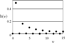
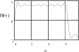
The filter impulse response used in this example (shown for positive ν only in the graph) is:

	Filter Impulse Response

 
h(ν) = k/ν for odd ν, and
h(ν) = 0 for even ν

	Filter Transfer Function

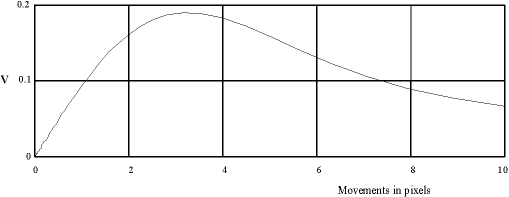
Using the above filter on data with a Gaussian form of autocorrelation function with RMS correlation length of 2.5 pixels the following results are obtained.

	Movement Calibration

 

	Root Power Spectra of Movement Error

**    Discussion

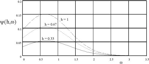The form of the errors.

The form of the transmission characteristic is an S-shape, similar to that of a phase discriminator, of which it is a generalised case. The amplitude of the inherent noise produced by the process varies essentially in proportion to the magnitude of movement being measured over the useful portion of the transmission curve. This noise is strongest at spatial frequencies between 0.5 and 1 cycles per pixel.

Interference between superposed signals.

If the image is composed of superposed components moving with differing speeds then the resulting output from the measurement process will be a single result which does not necessarily represent well any particular component. The output from the product summation process is proportional to the variance of the original image, and this can be compensated by dividing by the measured total variance. When two components add in the image then so long as they are uncorrelated images then their respective mean outputs will remain unchanged; there will be more noise present. The output will then be a single value which is the sum of the two independent terms weighted in proportion to their respective image variances.

Choice of filter.

The example shown above uses an approximation to the ideal filter with constant sensitivity across the range of spatial frequencies in the image. If the filter is simplified to the extent of making it as simple as possible then it involves only the terms at the two adjacent pixel positions. When this is done then the sensitivity for the system will vary inversely with the RMS correlation length of the image.

**    References and Background Reading

[ABo01]	A.G.Booth "Rotation Measurement by Optical Speckle."
[BM87]	Y.Bresler & S.J.Merhav "Recursive Image Registration." IEEE Trans Ac.Sp.&Sig.Proc ASSP-35 No1 Jan 87 pp70-85
[EH79]	E.L.Hall "Computer Image Processing & Recognition." New York: Academic 1979 pp480-554 This book not yet seen by AGB.
[HM76]	H.Meyr "Delay Lock Tracking of Stochastic Signals." IEEE Trans Commun COMM-24 Mar 76 pp331-339
[HP94]	H.V.Poor "An Introduction to Signal Detection and Estimation." 2nd.Ed. 1994 Springer-Verlag.
[HS81]	Horn & Schunk "Determining Optical Flow." Artific. Intell. V16 May 81.
[JB64]	J.F.Barrett "Hermite Functional Expansions and the Calculation of Output Autocorrelation and Spectrum in any Time-Invariant Non-linear System with Noise Input." J.Electron.Control. V16 No.1 1964, pp107-113
[OM93]	"Optical Methods in Engineering Metrology." Ed. D.C.Williams Chapman & Hall 1993 ISBN 0-41-239640-8
[RB89]	S.J.Rothberg,J.R.Baker,N.A.Halliwell Letter:"Laser Vibrometry: Pseudo-Vibrations." Jour.Sound&Vibration 1989 135(3) pp516-522
[RH94]	S.J.Rothberg,N.A.Halliwell "Vibration Measurements on Rotating Machinery using Laser Doppler Velocimetry." Trans ASME Jul 94 V116 pp326-331
[RT92]	M.Reynolds,V.Toal "An Interferometric Linear In-plane Position Transducer." Optics&Laser Technology. 1992 V24 N2 pp59-65
[SM61]	J.J.Spilker & D.T.Magill "Delay Lock Discriminator - an Optimum Tracking Device." Proc IRE V49 Sep 61 pp1403-1416
[WD75]	R.F.Webber & W.H.Delashmit "Product Correlator Performance for Gaussian Random Scenes." IEEE Trans Aerosp.Electron.Syst AES-10 Jul 75 pp516-520
[YF91]	I.Yamaguchi,T.Fujita "Linear and Rotary Encoders using Electronic Speckle Correlation." Jour.Opt.Eng. 1991 V30 N12 pp1862-1868
[ZH67]	Y.Zhang & M.T.Hagan "A Reduced Parameter Bilinear Time Series Model." IEEE Trans Sig Proc V42 No7 pp1867-1870